Section 6: Smart Labeling Service for Object Detection
AI-Assisted Data Labeling for Every Research Domain
This tutorial walks through the Smart Labeler object detection workflow, from opening the demo pipeline to producing a classified, exportable set of annotations. Smart Labeler pairs manual annotation tools with AI-assisted detection (SAM 3, OWLv2) and embedding-based classification (BioCLIP 2, DINOv3) so that large image datasets can be labeled quickly and then reviewed rather than labeled entirely by hand.
Contents
- Stage 6.1: Getting Started
- Stage 6.2: Annotation
- Stage 6.3: Build Class Supports
- Stage 6.4: Optimize Patch Size
- Stage 6.5: Configure and Run Detection
- Stage 6.6: Classification
Stage 6.1: Getting Started
Step 6.1.1: Open Smart Labeler
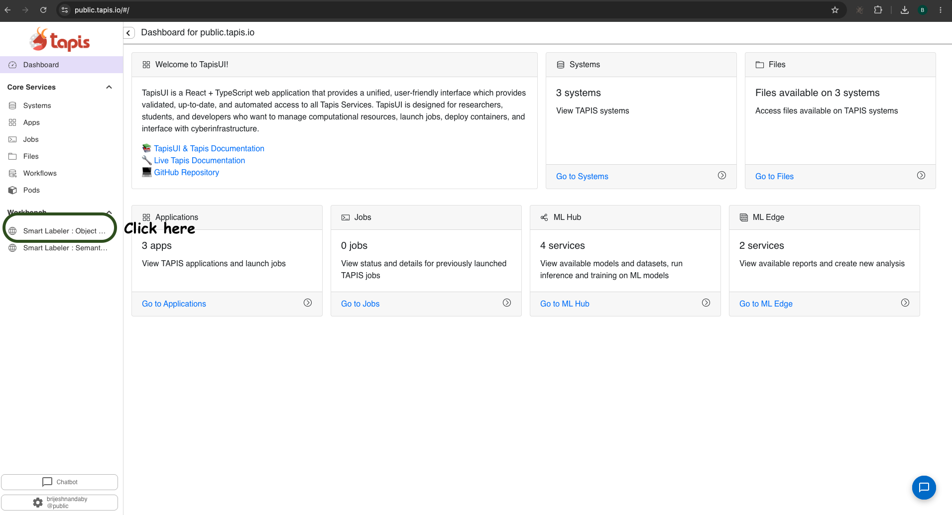
Log in to https://public.tapis.io/, then click on the service as shown below.
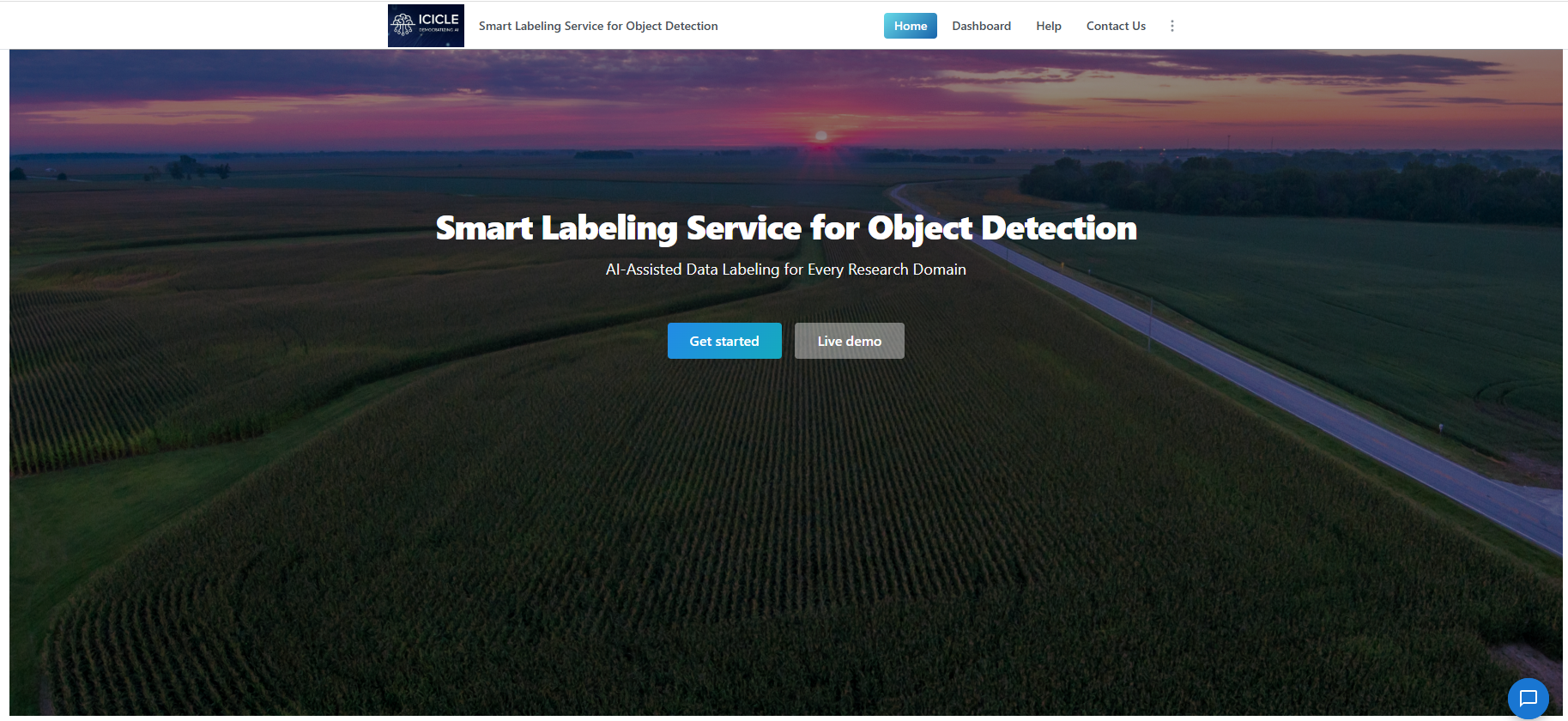
Navigate to the Smart Labeler. The landing page introduces the service and gives you two entry points: Get started, which takes you into your own pipelines, and Live demo, which opens a pre-loaded pipeline you can explore without uploading any data.
Step 6.1.2: The Pipelines Dashboard
Every dataset you annotate lives inside a pipeline. The Pipelines dashboard lists all pipelines you have access to, including a Demo Pipeline at the bottom that comes pre-loaded with data so you can try the full annotation workflow without any setup.
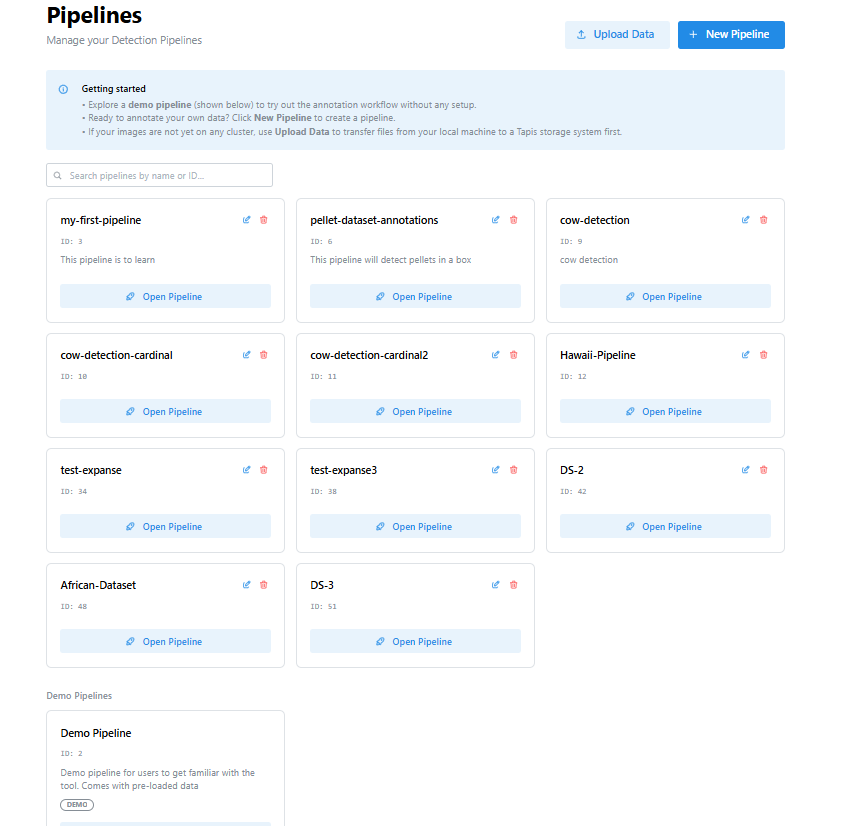
A few things worth noting on this page:
- Use the search bar to find a pipeline by name or ID.
- Each pipeline card shows an Open Pipeline button, plus edit and delete icons.
- If your images aren’t yet on a Tapis-managed cluster, use Upload Data first (Step 1.3).
- To start annotating a brand-new dataset, use New Pipeline (Step 1.4).
Step 6.1.3: Upload Data to Tapis
If your images live on your local machine, click Upload Data from the Pipelines dashboard. This opens a dialog where you select the target Tapis storage system and destination path, then either drag and drop files or use Select Files / Select Directory to choose what to upload.
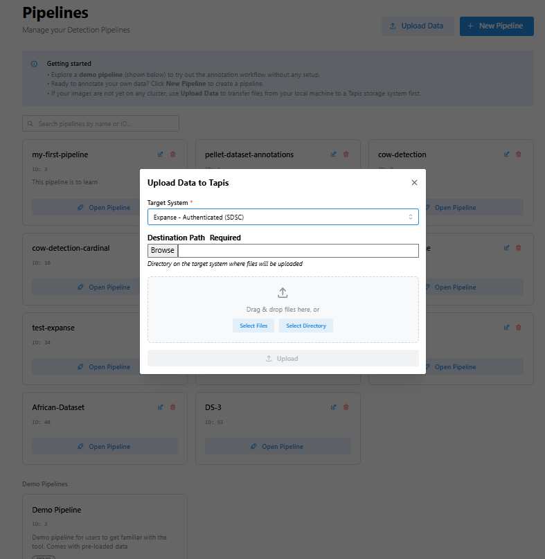
Once the upload finishes, your images are available on the target system and can be referenced when you configure a pipeline or a detection job later in this tutorial.
Step 6.1.4: Create a New Pipeline
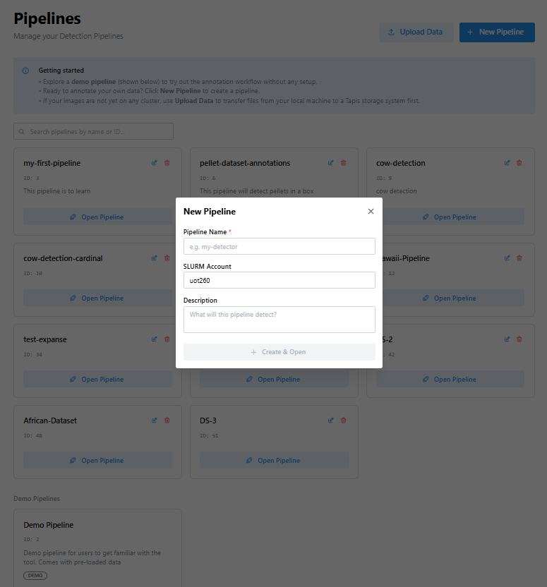
Click New Pipeline to create a pipeline for your own dataset. Give it a Pipeline Name, confirm the SLURM Account used for compute jobs, and optionally add a Description so collaborators know what the pipeline is for.
Here’s the same dialog filled out for a pipeline that verifies dog breed annotations:
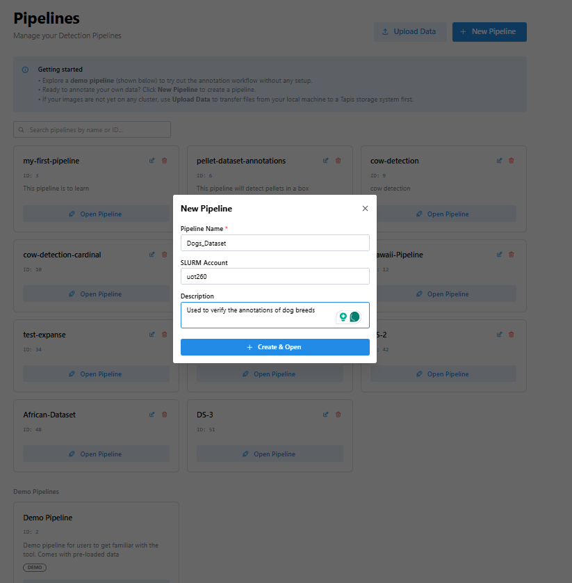
Click Create & Open to create the pipeline and jump straight into the Annotation stage.
Stage 6.2: Annotation
Opening a pipeline drops you into the Image Annotator, the first stage in the pipeline breadcrumb at the top of the screen. This is also where you’ll return later to review and correct AI-generated detections.
Step 6.2.1: The Image Annotator Layout
The Image Annotator is split into three areas: the File Explorer on the left (collapsed by default), the image canvas in the center, and the annotation controls on the right. The pipeline breadcrumb across the very top always shows which stage you’re in — Annotation is active here, with every later stage listed to the right of it.
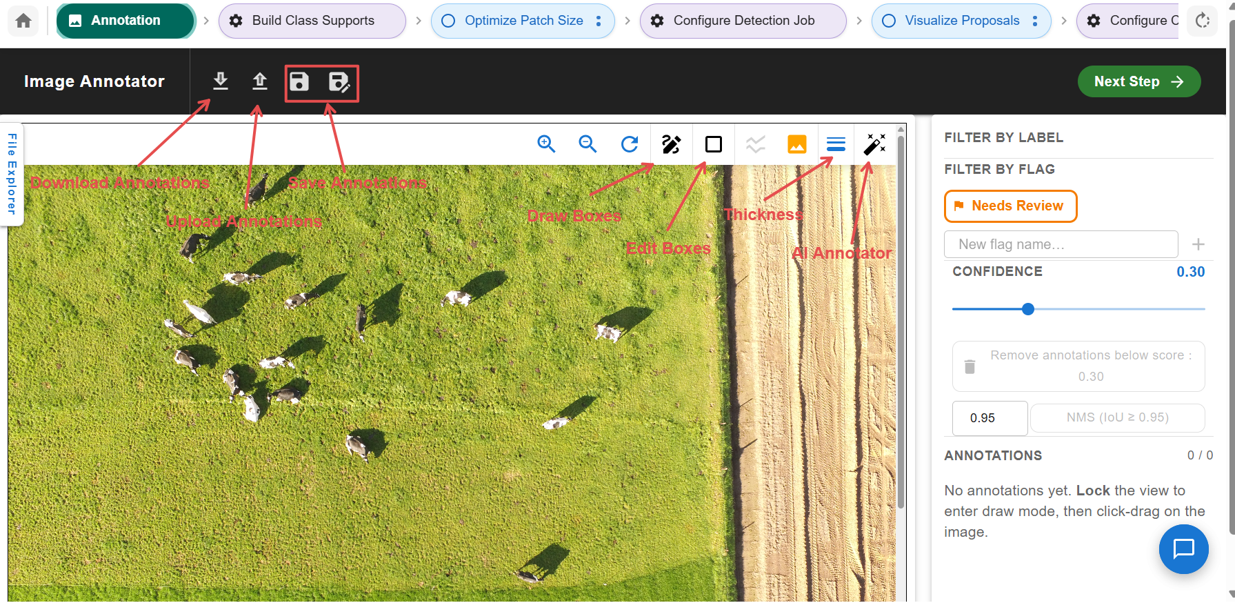
Across the top toolbar:
- Download Annotations and Upload Annotations — export or import an annotation file directly from this view.
- Save Annotations and the adjacent icon — save your current annotations to a Tapis file path.
- Draw Boxes — switch into manual bounding-box drawing mode.
- Edit Boxes — select and adjust existing boxes.
- Thickness — change the line weight used to render boxes.
- AI Annotator — open the SAM 3 segmentation-assisted annotation dialog (covered in Step 2.4).
Step 6.2.2: Browsing Images with the File Explorer
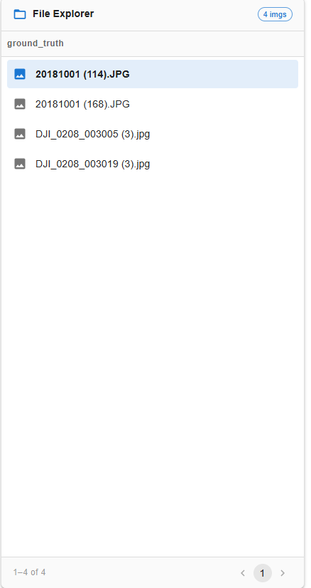
Click the File Explorer tab on the left edge of the Annotator to expand it. It lists the images available in the current pipeline’s source folder, along with pagination controls at the bottom. Click any thumbnail or filename to load that image into the canvas.
Step 6.2.3: Zero Shot Annotation and Filtering Tools
The right-hand panel gives you fine-grained control over which annotations are visible and lets you manage them individually.
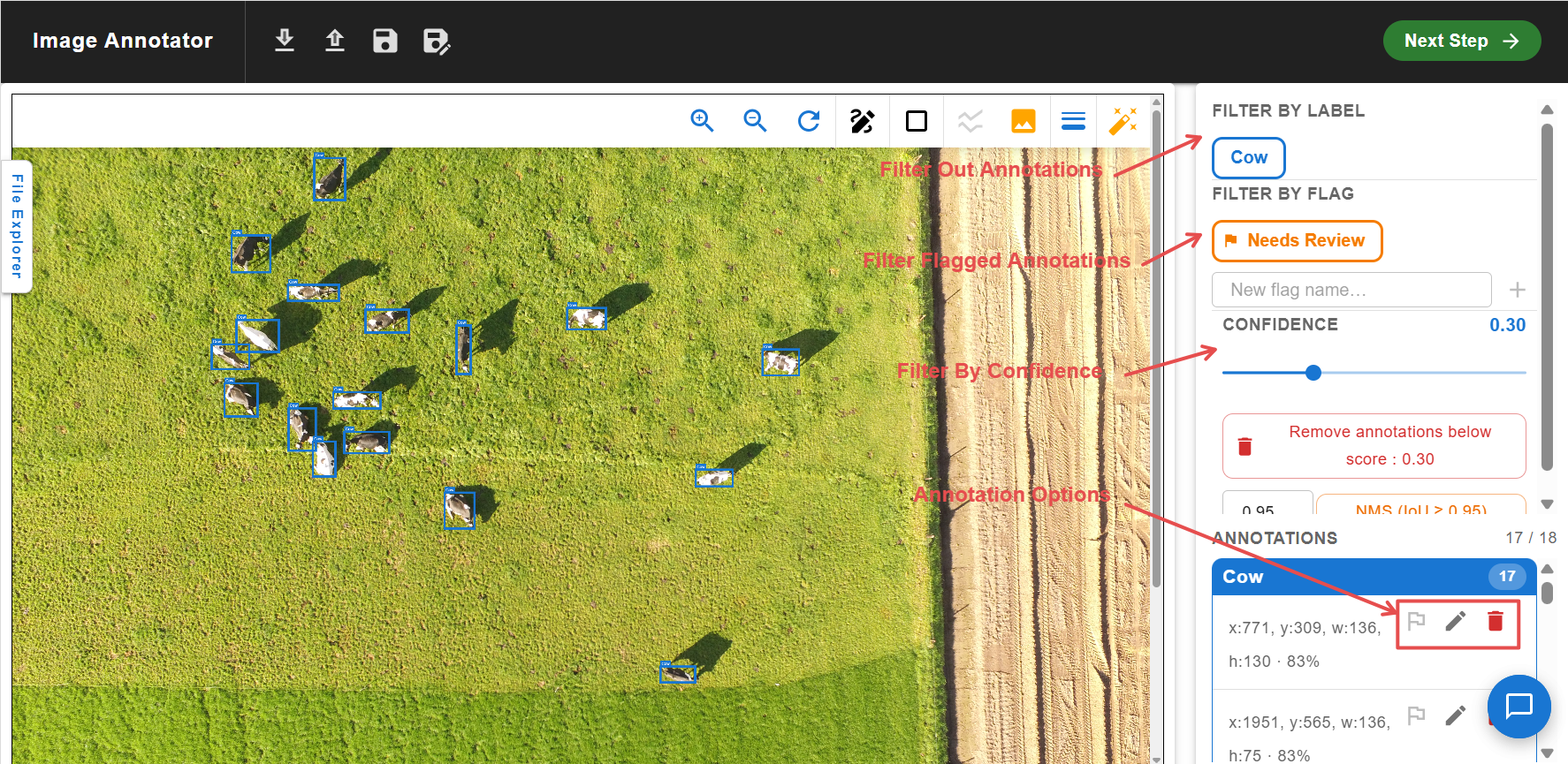
- Filter by Label — toggle visibility of annotations by class (e.g.
Cow). - Filter by Flag — show only annotations you’ve flagged, such as Needs Review. You can also define your own custom flags.
- Filter by Confidence — use the slider to hide low-confidence detections, and use Remove annotations below score to delete them outright.
- Annotation Options — each row in the annotation list has its own flag, edit, and delete controls, so you can review detections one at a time.
The list at the bottom shows every annotation for the current image, with its bounding box coordinates and confidence score, grouped by class.
Step 6.2.4: AI-Assisted Annotation with SAM 3
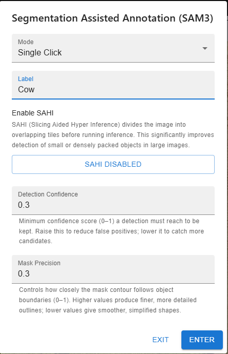
Rather than drawing every box by hand, you can click the AI Annotator icon to open the Segmentation Assisted Annotation (SAM 3) dialog. SAM 3 supports two modes:
Single Click mode lets you label one object at a time. Set the Label you want applied, then click directly on an object in the image; SAM 3 proposes a mask and bounding box around it.
Text Prompt mode detects every instance of a class across the whole image from a text
description alone — no clicking required. This is the fastest way to bulk-annotate a common
class like Cow.
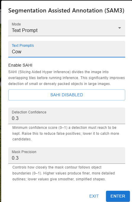
Both modes share the same tuning controls:
- Enable SAHI — Slicing Aided Hyper Inference splits the image into overlapping tiles before running inference, which significantly improves detection of small or densely packed objects in large images.
- Detection Confidence — the minimum confidence score a detection must reach to be kept. Raise it to reduce false positives, lower it to catch more candidates.
- Mask Precision — how closely the mask contour follows object boundaries. Higher values give finer, more detailed outlines; lower values give smoother, simplified shapes.
Click ENTER to run the detection and populate the canvas with proposed annotations, which you can then review using the filtering and editing tools from Step 2.3.
Step 6.2.5: Saving, Importing, and Downloading Annotations
Once you’re happy with a set of annotations, click the Save Annotations icon in the toolbar. Choose the target Tapis system and enter a File Path, or toggle Default JSON to switch the export format. A Format Preview shows exactly what the saved file will look like before you commit.
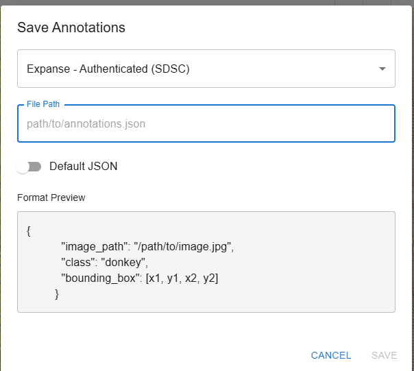
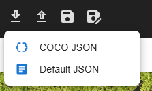
The Download Annotations icon offers a quick local export in either format:
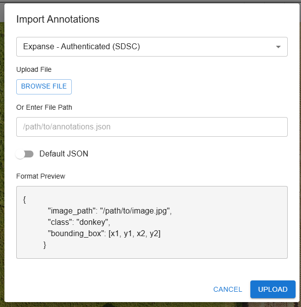
To bring in annotations you’ve already created elsewhere — for example, ground-truth labels you want to compare against — use Upload Annotations. You can browse for a local file or point to a file path already on the target Tapis system, and the same Format Preview confirms the expected structure before upload.
Stage 6.3: Build Class Supports
Once you have a set of labeled reference examples, the next stage generates class support embeddings — reference feature vectors for each class that the detection and classification jobs later compare new proposals against.
Step 6.3.1: Generate Class Supports
From the pipeline breadcrumb, open Build Class Supports. Fill in:
- Job Name — a descriptive name for this run.
- System — the compute system the job will run on.
- Source Image Directory, Annotation File Path, and Output Directory — browse to or type the full paths for your labeled images, their annotation file, and where results should be written.
- Model Selection — choose one or more embedding models. In this run, BioCLIP 2, DINOv3 ViT-S/16, and OWLv2 Large Patch14 Ensemble are all selected; selected models are listed for confirmation below the picker.
- Crop/Patch Size — the pixel dimensions used when cropping each labeled object for embedding.
- Device and Method — select the compute device and processing method (e.g.
Image).
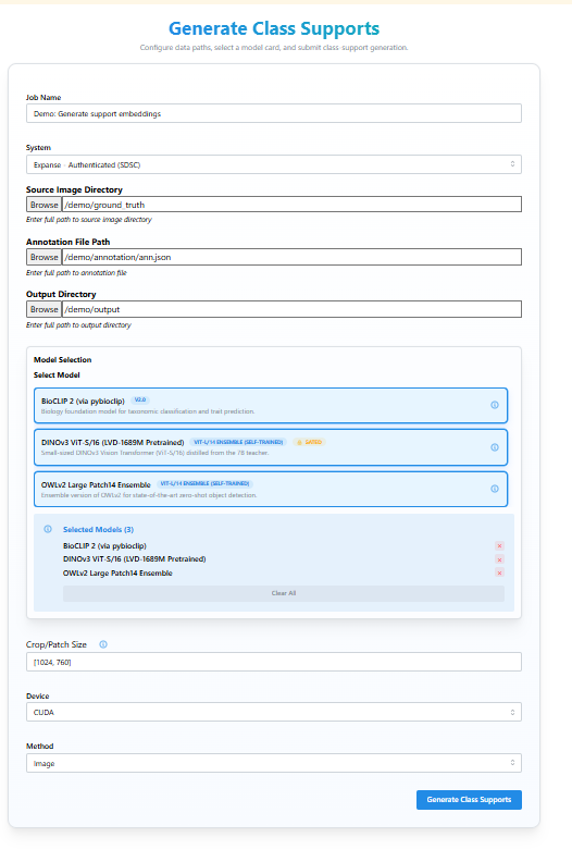
Click Generate Class Supports to submit the job. The resulting embedding files are what you’ll reference in Stage 5 when configuring the detection job.
Stage 6.4: Optimize Patch Size
Detection accuracy on aerial or wide-angle imagery is sensitive to the crop size used during inference — too large and small objects get lost, too small and context is lost. The Optimize Patch Size stage lets you compare candidate crop sizes side by side on real imagery before committing to one.
Step 6.4.1: Compare Crop Sizes
Each entry under Class Supports Files corresponds to a job that was run with a different
crop size (for example, 314, 960, 1024, and 2500 pixels). Select an entry to overlay
its resulting boxes on the canvas, adjust the crop size field, and click Re-submit Job to
try a new value. Once you’re satisfied with a size, click Save to carry it forward.
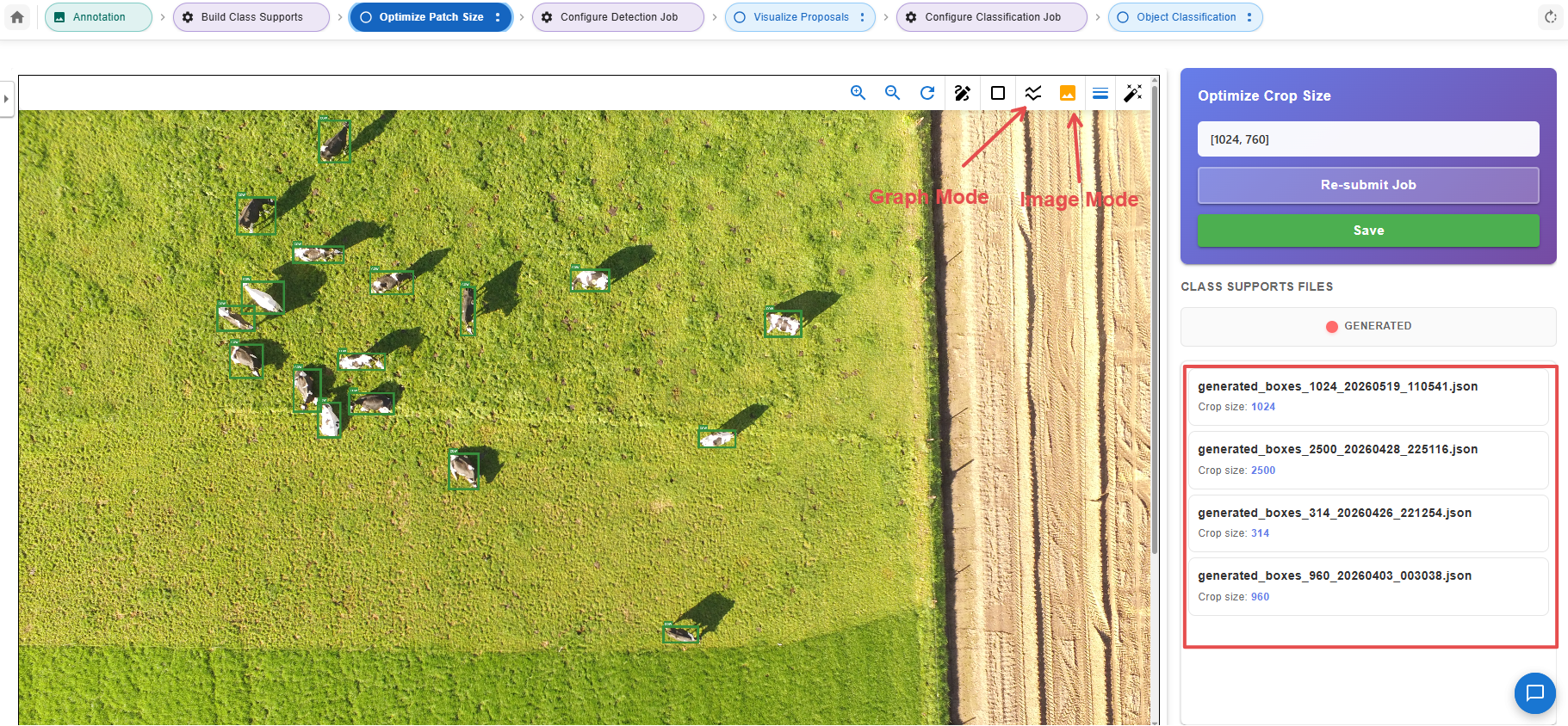
In this example, a crop size of 1024 produces well-fitted boxes around each cow in the
field — a good sign that this value balances detail against context for this dataset.
The toolbar above the canvas also includes an Image Mode / Graph Mode toggle. Image Mode is the visual overlay shown above; switching to Graph Mode instead plots an IoU Score against each annotation for every candidate crop size, letting you compare accuracy quantitatively rather than by eye alone.
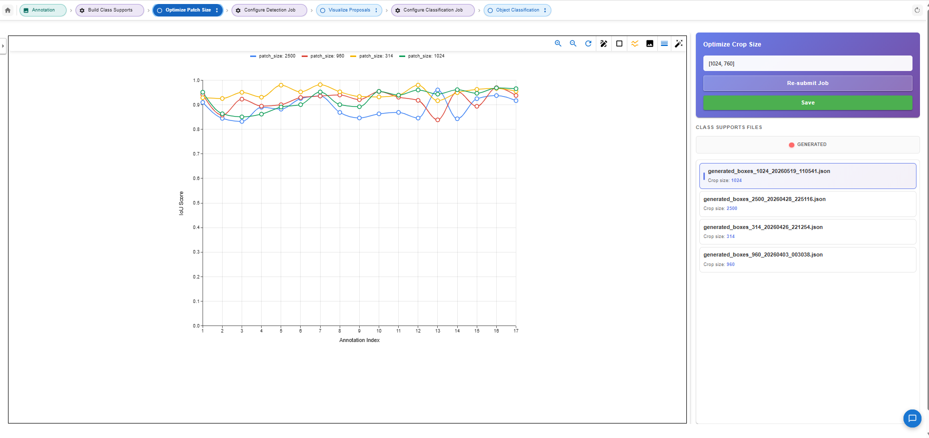
Here, patch_size: 314 (yellow) tracks consistently higher IoU scores across most
annotations than the other candidates, while patch_size: 2500 (blue) dips lowest —
useful confirmation to weigh alongside the visual comparison before clicking Save.
Stage 6.5: Configure and Run Detection
Step 6.5.1: Configure the Detection Job
Open Configure Detection Job from the breadcrumb. The left panel defines the job:
- Job Name and Training System — name the run and pick the compute system.
- Query File Location and Output Directory — the directory of images to run detection on, and where results should be written.
- Model Selection — pick one or more Proposer models (models that generate candidate boxes, such as OWLv2 Large Patch14 Ensemble and Segment Anything Model 3) and, further down the form, one or more Embedder models used for classification support.
The right panel, Saved Configurations, lets you reuse a previous setup — click a saved card to load its models, thresholds, and settings instantly instead of re-entering them.
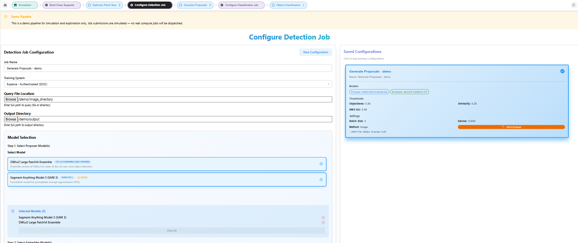
The selected configuration here uses the SAM3, OWLv2-Ensemble proposer pair together with
the BioCLIP 2, DINOv3 ViT embedder pair, an objectness threshold of 0.25, a similarity
threshold of 0.20, NMS IoU of 0.50, batch size 4 on CUDA, with SAHI enabled at a
640px tile size and 0.25 overlap — the same SAHI tiling behavior introduced in Step 2.4,
now applied at the batch job level.
Scrolling down completes the rest of the form: Step 2: Select Embedder Model(s) (the same picker pattern as the proposer models above), Advanced Settings (Batch Size, Device, Method, and the SAHI tile size / overlap ratio fields), Detection Thresholds (Objectness, Similarity, and NMS IoU), and HPC Resource Settings (Node Count, Cores Per Node, Memory, and Max Minutes) for the compute job itself.
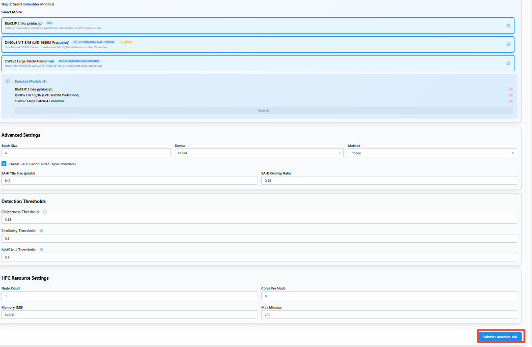
Once every field is set, click Submit Detection Job to launch the run.
Step 6.5.2: Visualize Proposals
After the detection job completes, open Visualize Proposals to review what the models found. The canvas shows each proposed box, and the right panel summarizes the exact job configuration that produced them.
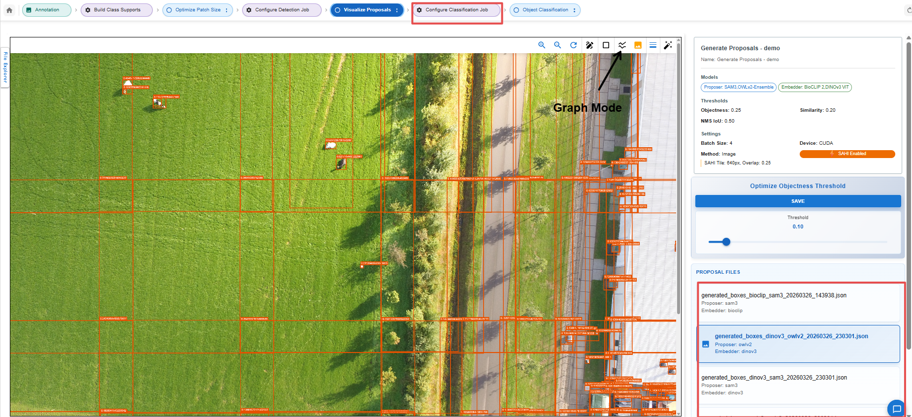
The orange grid overlaying the image shows the SAHI tiles the detection job sliced the image
into before running inference — a direct visual of the 640px tile size and 0.25 overlap
configured in Step 5.1. The Graph Mode toggle in the toolbar switches this same canvas to
a plot instead of an image overlay.
The Proposal Files list on the right shows one result file per proposer/embedder
combination — here, sam3 + bioclip, owlv2 + dinov3, and sam3 + dinov3. Select a
file to load its detections into the canvas above. An Optimize Objectness Threshold
slider sits just above the list, letting you raise or lower the cutoff and immediately see
which proposals survive.
Switching to Graph Mode plots Objectness Score against every detected proposal, sorted from highest to lowest confidence:
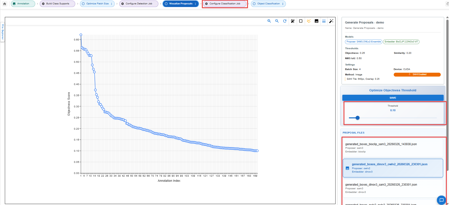
The sharp drop-off partway through the curve is a useful signal for where a sensible objectness threshold sits — proposals to the left of the knee are confident detections, while the long, low-scoring tail to the right is mostly noise worth filtering out before moving on to classification.
Stage 6.6: Classification
With detection proposals in hand, the final stage assigns each proposed box a class label by comparing it against the class support embeddings built in Stage 3.
Step 6.6.1: Configure the Classification Job
Open Configure Classification Job. Set a Job Name and confirm the System, then tune:
- Similarity Threshold and Objectness Threshold — matching thresholds between 0 and 1 that control how confidently a proposal must match a class support before it’s labeled.
- Proposal & Class Support Mapping — click Add Mapping to pair each proposal tensor file (the output of Stage 5) with its associated class support file (the output of Stage 3). If the detection job is still running, the proposal file will simply appear here once processing completes.
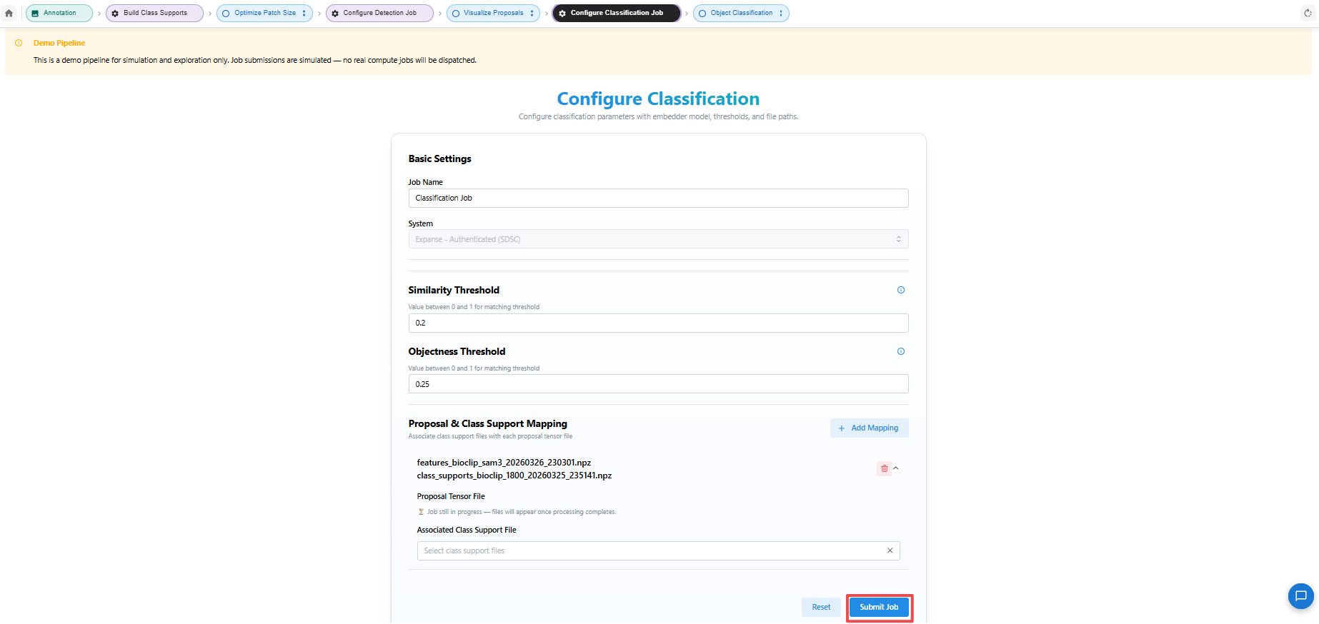
Click Submit Job to run classification across all mapped proposal files.
Step 6.6.2: Review Object Classification Results
Once classification completes, open Object Classification, the final stage in the breadcrumb, to see the fully labeled result. Each detected object is now outlined and tagged with its assigned class directly on the image.
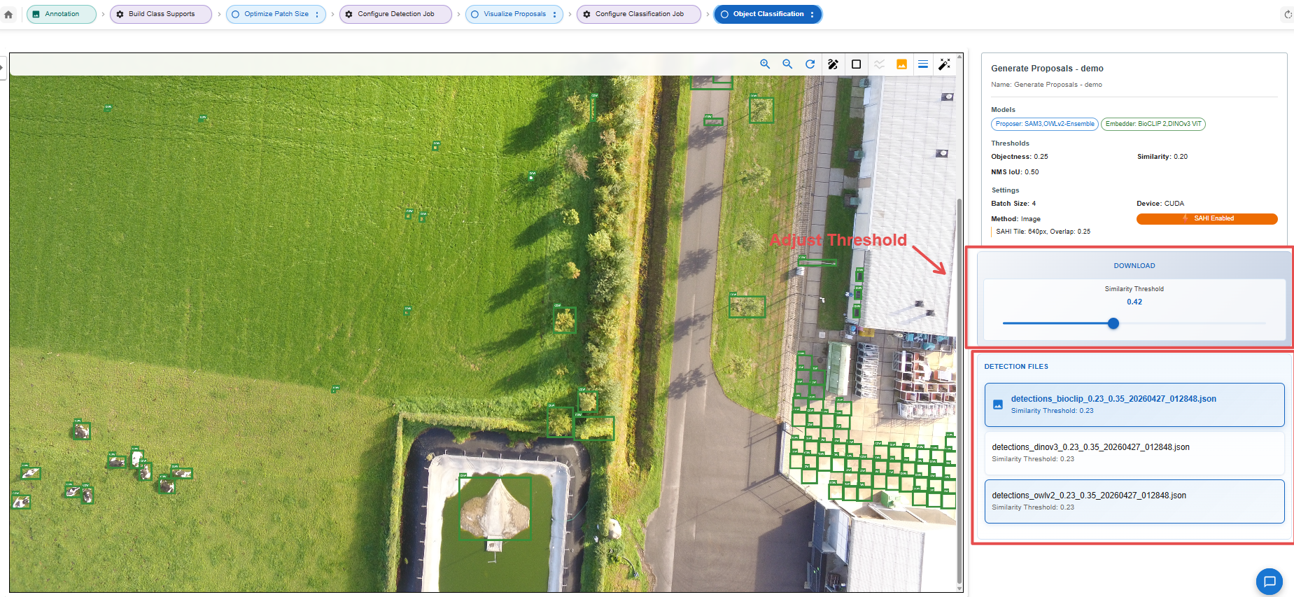
The right panel still shows the originating job configuration (models, thresholds, and settings), along with a Download section and a Similarity Threshold slider you can adjust to tighten or loosen which classified detections are shown, plus the same Detection Files list from Step 5.2 so you can compare results across models before exporting.
From here you can return to the Annotation stage at any point to spot-check individual detections, apply the Needs Review flag to anything questionable, and correct or delete boxes before exporting your final annotation file using Save Annotations or Download Annotations (Step 2.5).
This completes the end-to-end Smart Labeler workflow: annotate a seed set of examples, build class supports, tune your patch size, run and visualize detection proposals, classify them, and review the results — turning a handful of manually labeled images into a fully annotated dataset with AI assistance at every step.
Launching the Jupyter Notebook Environment
Jupyter is an open source project that provides a webapp interface for writing code and documents. Throughout this tutorial, we will be using a Jupyter Notebook environment for making Tapis User Requests.
To evaluate the model, start up your Jupyter Notebook Environment
Login with TACC credentials on TACC’s Public JupyterHub
Navigating to the $WORK File System
On successful login, you should see a ai-tutorial-2026 folder, within the Jupyter file system.
Restarting your Jupyter Server
Click on Files -> Hub control panel -> Stop my server -> Start server